The Python codes I wrote for creating the animations in this post are available at my github repo.

Like Archimedes, I like my occasional warm bath in winter. And like Archimedes, I am given to pensive cogitations in the bath tub. On one such occasion, spent in pensively reflecting and cogitating in the bath tub on this and that, the patterns of waves on the water surface caught my attention. The slightest movement on my part would set off a wave in motion, which would go out in a circle, get reflected from the wall of the tub, change direction, come back, meet another wave coming in from the other direction, get reflected from the opposite wall, and so on it went, getting reflected over and over again, meeting other waves on the way, which in their turn were being reflected and traveling back and forth, till in the end an absolutely incomprehensible display of patterns developed itself in the bath tub. “a fascinating display of shimmering patterns” is another way to describe the phenomenon. I accordingly transferred my cogitations to understanding these patterns. After the mechanism was clear, I spent some time in coding with Python to simulate them, and here is the result of that simulation:

Fig. 1

And I thought, why stop with a square boundary with the source at the center, why not do it for a recangular boundary as well with the source at an arbitrary point? Well, I modified the program a bit, and this is what the simulation looks like:

Fig. 2

In this post I'd like to share how the above animations were created as well as the physics of the above phenomenon.

During my initial searches on Google, I did not find much regarding wave reflection from multiple boundaries, which was surprising because it is a very good illustration of how very simple ideas can lead to quite complicated looking phenomena. In fact, the basic idea is quite simple and is based on the reflection of a one dimensional wave from a single boundary. So let us revisit this concept.

Reflection of one dimensional waves at a boundary¶

I had read about the reflection of one-dimensional waves at a boundary from the Feynman lectures on physics (FLP) when I was a physics student. It was a long time ago, but it seems like yesterday when I was sitting in the bus and reading about it. And I distinctly remembered the mechanism, since it was so simple in its essence.

The system being considered was a rope fixed at one end with a pulse traveling along its length. (In the following I have used the words “pulse”, “wave” and “wave form” interchangeably.) The question was to understand how the pulse would be reflected from the fixed point when it reached there. It turns out that due to the nature of the wave equation and the boundary condition in this case, this reflection can be thought of as a linear combination of two virtual waves: one wave traveling in the positive direction and the other in the negative direction, and the actual wave is a superposition of the two. (see here for the explanation from the online version of FLP.) It is almost as if an imaginary wave is coming from the other side of the fixed point and meeting the actual pulse at the fixed point, and the two pulses then go along the way. I created some animations to illustrate the idea. The first of these shows just the process of reflection without the virtual waves:

Fig. 3

It shows a wave pulse traveling on a rope fixed to a wall and and as it reaches the wall it gets reflected into the other direction.

As mentioned earlier this can be thought of as a combination of two virtual waves traveling in opposite directions. The next animation below shows the actual wave along with the two virtual wave forms. The actual wave form (red) is a superposition of the virtual (blue and green) wave forms.

Fig. 4

The one in blue is a waveform traveling to the right and the one in green is traveling to the left and the actual wave form is a superposition of both. Except for a sign change, the two are mirror images of each other, which is required to ensure that the end point of the string remains fixed to the wall at all times. (The particular waveform I have chosen is such that the two wave forms overlap only when they reach the wall, and hence the actual wave form will resemble the blue one before reflection and the green one after reflection. Only during the reflection process it will look somewhat different due to the overlap. In general the two virtual waveforms may always have considerable overlap and thus the actual waveform may bear little resemblance to the virtual waves. For example, a standing wave on a string fixed at both ends is a superposition of a virtual wave traveling in the positive direction and a virtual wave traveling in the negative direction, but the standing wave itself has little resemblance to either of the virtual waveforms.)

What I find really intriguing is that it is almost as if an imaginary wave is coming from the other side of the fixed point and meeting the actual pulse at the fixed point, and the two pulses then go along the way.

Formally, the blue waveform, being a wave traveling in the +x direction, can be expressed as $f(x–vt)$, where $v$ is the speed of the wave and $t$ is the time. The point where the rope is attached to the wall is $x = 0$. Similarly, the green waveform, being a wave traveling in the $-x$ direction and being the inverted mirror image of the blue one, is $-f(-x–vt)$. Hence the actual wave, shown in red, is $u(x,t) = f(x–vt)-f(-x–vt)$. This ensures that the point where the string is attached to the wall remains fixed at all times.

What happens when, instead of being rigidly fixed to the wall, the end of the string is allowed to move freely at the boundary without resistance? In this case, assuming the rope is massless, the slope of the tangent at the end point of the string must always be zero. This is ensured by requiring that the virtual waveforms be mirror images of each other. Under this condition the actual waveform becomes $u(x,t) = f(x–vt)+f(-x–vt)$. The partial derivative of $u(x,t)$ with respect to $x$ at $x = 0$, which is the slope of the tangent at the end point of the string, is indeed easily seen to be zero. The following animation shows this case:

Fig. 5

Reflection of two-dimensional waves at a boundary¶

The above explanation pertains to one-dimensional waves and for a single reflection at a boundary. As mentioned earlier, I wanted to understand multiple reflections for a two-dimensional wave and eventually to simulate them. Before doing so I’d like to mention some simplifying assumptions about water waves in two dimensions which render the calculations tractable.

Some simplifications for water waves¶

At the outset I must mention some uncomfortable facts about water waves. Although waves on a water surface look so much like ordinary transverse waves, they are much more complicated. Feynman makes it clear that

“Now, the next waves of interest, that are easily seen by everyone and which are usually used as an example of waves in elementary courses, are water waves. As we shall soon see, they are the worst possible example, because they are in no respects like sound and light; they have all the complications that waves can have.”

For example, one may expect that a water molecule on the surface of a water wave executes up-and-down simple harmonic motion, just like in a transverse wave. However this picture is immediately seen to be wrong when one remembers that water is incompressible in the everyday world, and such a transverse motion would require that water be compressible. As Feynman goes on to say,

“What actually happens is that particles of water near the surface move approximately in circles. When smooth swells are coming, a person floating in a tire can look at a nearby object and see it going in a circle. So it is a mixture of longitudinal and transverse, to add to the confusion. At greater depths in the water the motions are smaller circles until, reasonably far down, there is nothing left of the motion.”

The following is a diagram from FLP, showing how the water molecules move on a water wave.

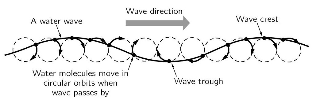
Fig. 6

Here is a very nice animation showing the motion of water molecules under the effect of a water wave, which is taken from this site. For a hardcore mathematical treatment of this fascination subject check out this book.

Regardless of the above complications it is however a matter of observation that the height of the water surface indeed behaves like a transverse wave, and I shall therefore assume that it satisfies the two-dimensional wave equation:

\begin{equation} \frac{\partial^2 h }{\partial x^2} + \frac{\partial^2 h }{\partial y^2}= \frac{1}{v^2}\frac{\partial^2 h }{\partial t^2} \end{equation}

I am interested in examining cylindrically symmetric solutions of the above equation. Before doing so it is useful to take a look at solutions of the one-dimensional wave equation and spherically symmetric solutions of the three dimensional wave equation. The solutions for these cases have a very nice and simple form and are intuitively simple to understand. So, in one dimension, for any arbitrary functions $f$ and $g$, $u(x,t) = f(x–vt)+g(x+vt)$ is a solution of the wave equation. This can be easily verified by substituting it in the one dimensional wave equation.

For spherically symmetric solutions in the three-dimensional case, the wave equation reads

\begin{equation} \frac{1}{r^2}\frac{\partial }{\partial r} \left( r^2 \frac{\partial h}{\partial r} \right)= \frac{1}{v^2}\frac{\partial^2 h }{\partial t^2} \end{equation}

By direct substitution it can be verified that $(1/r)[f(r-vt) + g(r+vt)]$ is the general solution of the above equation, in other words, the solutions are spherically symmetric waves traveling either towards the center or away from the center, with the amplitude proportional to $1/r$.

Hence in one dimension, the amplitude is independent of $x$, and in three dimensions the amplitude varies as $1/r$. Let us understand this physically. For simplicity let us assume that the functions $f$ and $g$ are sinusoidally varying functions. Let us further assume that the medium in which the wave travels consists of an infinite number of simple harmonic oscillators oscillating as the wave travels. In one dimension let the number of such oscillators per unit length be a constant $\lambda$. A small section of the rope of length $dx$ will thus have $\lambda dx$ oscillators. The energy of a simple harmonic oscillator is proportional to the square of its amplitude. Let the amplitude of each oscillator in this section $dx$ be $A(x)$. Since there are $\lambda dx$ oscillators, the total energy in length $dx$ is proportional to $λdxA(x)^2$. This should be independent of $x$ (This can be understood in various ways: either (1) by seeing that a sinusoidal function is linearly homogeneous, or (2) by physically assuming that someone is physically moving one end of the rope thus pumping in energy at a constant rate, so that in a section $dx$ of the rope, the energy that enters from the left must be equal to the energy that leaves from the right, otherwise there will be sinks or sources of energy, or (3) by considering a single pulse traveling across the rope and seeing that the number of oscillators per unit length is independent of $x$.) Since $\lambda$ is independent of $x$, it follows that $A(x)$ also must be independent of $x$.

What happens in the spherically symmetric three dimensional case? Well, let us assume that the number of oscillators per unit volume in space is a constant $\mu$. Consider a thin spherical shell of thickness $dr$ a distance $r$ away from the origin. The volume of this shell is $4\pi r^2dr$, hence the number of oscillators in this shell is $4\pi\mu r^2dr$. Let the amplitude of each oscillator be $A(r)$, implying the energy of each oscillator is proportional to $A(r)^2$. Multiplying this with the total number of oscillators in this shell gives us the total energy in this shell, which is thus proportional to $A(r)^2\cdot 4\pi\mu r^2dr$. Again, this must be independent of $r$, which is possible only if $A(r)$ is proportional to $1/r$.

Using a similar logic as above, one could conclude that the general solution for the cylindrically symmetric wave equation in two dimensions is $\rho^{-1/2} f(\rho–vt)$, where $\rho$ is the distance of a point from the $z$-axis in cylindrical coordinates. Indeed, a thin circular disc of thickness $d\rho$ and a distance $\rho$ away from the origin will have $\alpha\cdot 2\pi\rho d\rho$ number of oscillators, where $\alpha$ is the number of oscillators per unit area. If $A(\rho)$ is the amplitude of each oscillator in this disc, the total energy is proportional to $A(\rho)^2α2π\rho d\rho$, which again must be independent of $\rho$, suggesting that $A(\rho)$ varies as $\rho^{-1/2}$.

Unfortunately, this answer is wrong. This can be seen by explicitly substituting $\rho^{-1/2} f(\rho–vt)$ in the cylindrically symmetric two dimensional wave equation:

\begin{equation} \frac{\partial^2 h }{\partial \rho^2} + \frac{1}{\rho}\frac{\partial h }{\partial \rho}= \frac{1}{v^2}\frac{\partial^2 h }{\partial t^2} \end{equation}

This equation is not satisfied for the above form of the wave function. Indeed, there exists no $n$ for which $ρ^n f(ρ–vt)$ will satisfy the above equation. For, if you substitute

\begin{equation} h(\rho,t)=\rho^n f(\rho-vt) \end{equation}

in the above cylindrically symmetric two dimensional wave equation, an explicit calculation for the left hand side gives:

\begin{equation} \frac{\partial^2 h }{\partial \rho^2} + \frac{1}{\rho}\frac{\partial h }{\partial \rho} = n^2\rho^{n-2}f + (2n+1)\rho^{n-1}f' + \rho^n f'' \end{equation}

where $f'=\left. \frac{df(x)}{dx}\right|_{x=\rho-vt}$, $f''=\left. \frac{d^2f(x)}{dx^2}\right|_{x=\rho-vt}$, etc. This can satisfy the wave equation only when the first two terms (i.e. the $f$ and $f’$ terms above) vanish. The second term can indeed be removed by choosing $n = -1/2$, but the first term remains. (In contrast, for three dimensions the choice $n = -1$ satisfies the wave equation by eliminating the first two terms in the corresponding equation.)

However, for large $\rho$, the above guess does satisfy the wave equation, since in the large $\rho$ limit the first term also goes to zero. Hence the guess $\rho^{-1/2} f(\rho–vt)$ is strictly speaking a solution only in the large $\rho$ limit. The correct solution is given by the so-called Bessel functions, which indeed show an asymptotic $\rho^{-1/2}$ behavior in the large $\rho$ limit. (As an exercise one could try out the ansatz $g(\rho)f(\rho-vt)$ to see if an exact form for the amplitude $g$ can be found. This is physically more intuitive than the separation of variables method usually used.)

In our case we can always choose the boundaries at which reflection occurs to be so far away from the origin that the above asymptotic form for the amplitude holds.

Understanding multiple reflections of water waves in a square boundary¶

Having gained a bit of clarity regarding reflection of wave at a single boundary and the nature of the solution of the wave equation in one, two and three dimensions, it is time to come back to our original aim, viz. to understand multiple reflection of waves within an enclosed two dimensional region.

For simplicity, I decided to focus on a water surface enclosed in a square region and trace the multiple reflections of a single circular pulse starting from the center. From our discussion, the pulse, which is described by $f(\rho–vt)$, travels out at the speed $v$, and its amplitude falls off as $\rho^{-1/2}$. The function $\rho^{-1/2}f(\rho-vt)$ describes the height of the water above equilibrium at distance $\rho$ from the origin and at time $t$. I chose a Lorentzian form for $f(\rho-vt)$, although a Gaussian would have done as well. Thus if there are no boundaries, the height of the water above equilibrium at distance $\rho$ from origin and time $t$ is:

\begin{equation} h(\rho,t) = \frac{1}{\sqrt{\rho}} \cdot \frac{\eta}{(\rho-vt)^2+\eta^2} \end{equation}

where $\eta$ fixes the width of the pulse. The above just describes a circular pulse moving with velocity $v$ away from the origin. In the following animation the pulse is shown as a circle moving away from the origin.

Fig. 7

Now we come to the topic of reflections. The first step is to realize that the same principle which holds for one-dimensional waves holds for two dimensional waves as well. Hence the actual wave can be thought of as a superposition of two virtual waves. Let us consider reflection at a single boundary. Hence we have to consider the boundary as a mirror so the source which emits the pulse has its image which is . Also, open boundary conditions will be used. The following video shows the reflection of a circular pulse at a boundary.

Fig. 8

Now let us try to understand this in terms of virtual wave pulses. The following animation makes this clear.

Fig. 9

A gory application of the above is in maximising the damage caused by a nuclear explosion. When a nuclear bomb explodes above the surface of the earth, it sets out a spherical shock wave of highly compressed air at very high pressure. This wave after hitting the surface of the earth is reflected, like the above animation shows, and the region where the incident and reflected waves meet goes out in a circle, destroying everything in its wake. The reflected blast wave merges with the incident shock and forms what is known as a Mach stem. For reasons which have to do with the changes in temperature and pressure of the air caused by the explosion, this destruction is maximum when the bomb is detonated above a certain height from the earth’s surface and depends, among other factors, on the yield of the bomb. The Hiroshima bomb, which had a yield of about 16 kilotons of TNT, was exploded about 600m above the earth’s surface, while bombs with higher yield have a higher optimum height of detonation, sometimes even up to 3 to 4 km.

Coming back, we now have all the material required to understand multiple reflections in two dimensions from multiple boundaries. As mentioned earlier I’ll consider water confined in a square boundary with the wave pulse travel outwards from the center. If reflection takes place at all four boundaries of the square, we can expect, based on the above animation, that a virtual wave comes in from each side of the square, and each side of the square thus acts as a mirror. There are thus four additional virtual squares, one on top, one on bottom, one to the right, and one to the left of the real square. The motion of the virtual water in these virtual squares are exact mirror images of the water in the center square. However, and this is where it becomes really interesting, these four virtual squares are not enough – to track the movement of the reflected wave as it travels further, it becomes necessary to include four more virtual sources – one at NW, NE, SW and SE of the actual square. And suddenly it becomes clear that we in fact need an infinite array of such virtual squares to track the reflections of the original wave. The point of invoking this virtual lattice is to ensure that refection symmetry holds. One could well write an algorithm that ensures reflection symmetry without invoking this infinite virtual lattice, but in my opinion present method is simple to implement and is intuitively simple to understand.

With the explanation behind, time to present the animations. First, I will show only the actual wave and the actual region without showing the virtual waves and the virtual lattice. To keep the animation from becoming too bulky, I will show the wave pulse as a line plot instead of the color map shown in the first animation. Of course, the amplitude of the pulse falls off as the inverse square root of the distance from the center, as explained earlier.

So, here is the first animation:

Fig. 10

It looks quite complicated by itself. However, it is simpler to comprehend when the virtual lattice and the virtual wave forms are also shown. This I have done in the next animation:

Fig. 11

Obviously the virtual lattice extends to infinity in both directions, but I have shown just a 5×5 part of that, with the real square at the center (shown with thick edges). When a disturbance is made in the central square, it is as if simultaneously the same disturbance is made in each of the of the image squares, and it is as if each of these disturbances is travelling in a circle of ever increasing radius. However, the actual action is taking place at the thick square in the center, which is all that we observe in reality. And if you follow it closely, you will notice that the motion of the waves in it is exactly the same as that in the previous animation.

Hence each wall of the square acts like a mirror and the entire infinite lattice of the virtual image sources are just mirror images of the single point at the center. If ever there was a room of mirrors, this would be it.

Note also the fractal nature of the above. For example if you consider a bigger square whose side is three times the square of the unit square and consider reflections of the wave pulse on this square only, you will notice that it has exactly the same pattern which the reflections in the unit square have.

Here is a playlist on my youtube channel of these animations, which includes a longer version of the animation shown at the beginning of this post.

The above explanation deals with the case when the wave originates from the center of a square boudary. You will notice that the second animation in this post shows a rectangular region and the wave originates from a point which is not at the center of the rectangle. The idea for simulating this case remains exactly the same: just consider the boundaries to be mirrors and the wave motion then is a superposition of the real wave and the image waves.

Readers familiar with the "method of images" in Electrodynamics will immediately note the similarity between that method and the method described in this post. The success of this method hinges on the correct boundary conditions being produced by the images and the absence of any images in the region of interest.

A further question raised itself: can this method be used to simulate two-dimensional wave reflections in a general polygonal region? As a first step, I considered the simpler case of a semi-infinite angular region defined by two lines meeting at a point and making a certain angle with each other. Here is turns out that the method described here works only if this angle is an even part of $\frac{n}{m}\cdot360^{\rm o}$, where $n$ and $m$ are both integers and have no factors in common, and $m$ is an even integer. For those cases where $m$ is odd, the procedure outlined here, i.e., treating the boundaries as mirrors and introducing the corresponding images, unfortunately introduces an image inside the region of interest. Here for example is an animation I created for the case where the angle is $20^{\rm o}$, which is an eighteenth-part of $360^{\rm o}$.

Fig. 12

That’s it. Hope you had fun, and thanks for being all the way till here!