Introduction¶

Principle Component Analysis (PCA) is a tool in machine learning and data science applications to reduce the number of dimensions of a data set. The idea is to pick only those components which have the maximum variance and leave out the rest. This serves two purposes: one is that by leaving out unimportant features one can improve the efficiency of machine learning algorithms, and the second is that the reduced dimensionality helps in a better visualization of the data. This article seeks to offer a fairly rigorous treatment of the subject, but in the backdrop of an easy to grasp example so that the intuitive side is not lost.

Rotation matrix in two dimensions¶

As a bit of revision, the rotation matrix in two dimensions is recalled here, since we will it use it in the next section.

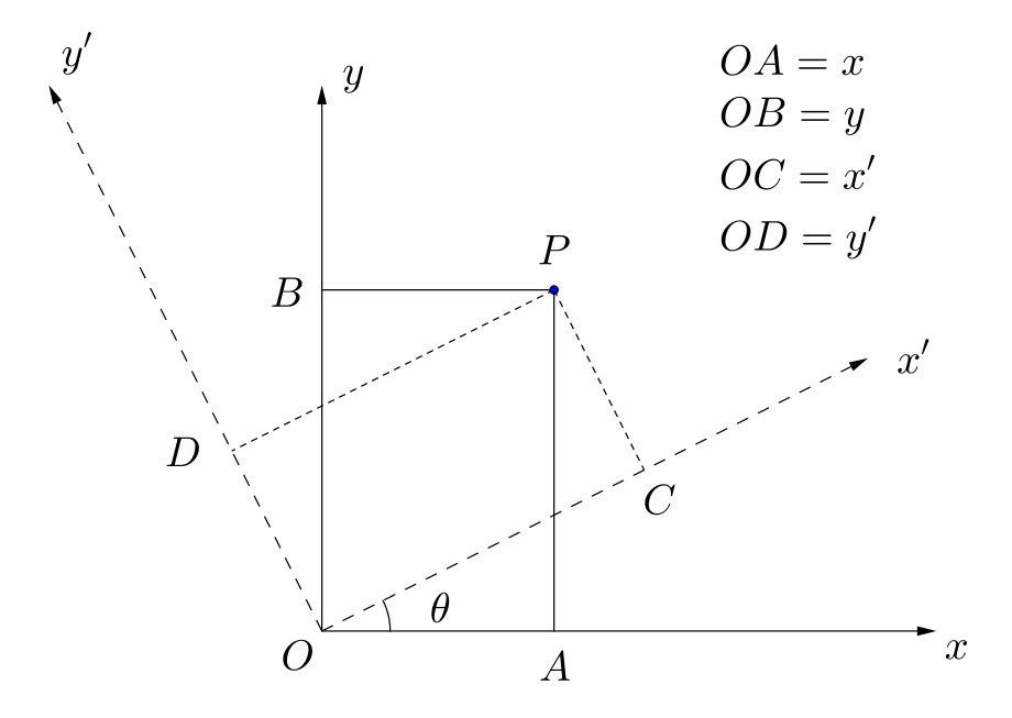
Suppose $x$ and $y$ are two features (they could be, for examle, the mpg and the weight features in the mtcars dataset). Consider a point P in $xy$ space with coordinates $x$ and $y$ (see the above figure, with $OA=x$ and $OB=y$). Now, keeping the origin fixed, we rotate the coordinate system in the anticlockwise direction by an angle $\theta$, and call the new coordinate system the $x'y'$ coordinate system. This is a special transformation of the coordinate system and is a pure rotation around the origin (there can be other transformations also: reflection, translation, scaling, etc. but we don't bother with them right now). In this new coordinate system, the coordinates of the same point P are $x'$ and $y'$ (in the above figure, $OC=x'$ and $OD=y'$). (FYI: this is a so-called passive transformation, in which the point remains fixed and the coordinate system is changed. In an active transformation, the coordinate system remains fixed but the point is moved.) The relation between the new rotated coordinates ($x'$ and $y'$) and the original coordinates ($x$ and $y$) of the point $P$ is then the following:

\begin{eqnarray} \left( \begin{array}{r} x' & \\ y' & \\ \end{array} \right)= \left( \begin{array}{rr} \cos\theta & \sin\theta \\ -\sin\theta & \cos\theta \end{array} \right) \left( \begin{array}{r} x & \\ y & \\ \end{array} \right) \end{eqnarray}

where the matrix on the right is the rotation matrix in two dimensions, which we shall call $R$. Using the fact that pure rotations do not change the length of the vector, it can be shown that $R$ is an orthonormal matrix, i.e. its transpose is its inverse (or equivalently, its inverse is its transpose): $R^TR=RR^T=I$.

In $p$ dimensions, the rotation matrix is $p\times p$ and is also orthonormal.

A two dimensional distribution of data¶

As a warm up let us consider the simple case of principal components in two dimensions for an artifically created data set. I will consider a distribution where the standard deviation for $x$ is $\sigma_x = 10$ and for $\sigma_y =3$, and $x$ and $y$ are independent (i.e. no correlation between the two). I also fix the mean of x and y at zero. The distribution for this case is

\begin{equation} P(x,y) = \frac{1}{2\pi \sigma_x\sigma_y}\cdot \exp\left[ -\frac{1}{2}\left( \frac{x^2}{\sigma_x^2} + \frac{y^2}{\sigma_y^2} \right) \right] \end{equation}

The above follows a joint normal distribution in $x$ and $y$. Now let us rotate the coordinate system by -30$^{\rm o}$.

And now let us plot it in the new ($x'y'$) system.

Now let us assume that this is the data we are working with, and have no idea how it was created. We also assume that our features are $x'$ and $y'$. The aim of PCA is to find a direction along which the variance is maximized. But what does this sentence actually mean?

Well, it means the following. Take any point P in the scatter cloud and consider its projection OB along the direction ${\hat u}$ (directed along the blue line). We now consider the variance of OB, i.e. we take each point P, find the corresponding projection OB, and find the variance of all these OB. Now our aim is to choose the blue line such that the variance of OB is maximum. If we find such a line, then we can replace all the points P by the points B, hence reducing the number of dimensions from 2 to 1.

In the above picture, we see that in the $x'y'$ system, choosing the unit vector along OB to be

$${\hat u} =\left( \begin{array}{r} \cos 30^{\rm o} \\ \sin 30^{\rm o} \end{array} \right)$$

gives the first principal component, that is, the variation along this direction will be maximum. Of course, it was easy in this case to find the direction of maximum variance, since there are only two dimensions and the rotation direction was chosen by ourselves. But we need a method for a general data set and higher number of dimensions. But the present simple case of two dimensions can nonetheless guide us to the answer.

The procedure for finding the direction of maximum variance (the principal component) is as follows:

• Find the expression for the variance along the direction ${\hat u}$.
• Find ${\hat u}$ so that the variance is maximized.

Expression for variance along the direction ${\hat u}$¶

Right now we stick to two dimensions and pretend that we do not know what the direction of maximum variance is. Suppose $x$ and $y$ are the coordinates of $P$, and $u_x$ and $u_y$ are the components of ${\hat u}$ (which in the previous section happened to be $\cos 30^{\rm o}$ and $\sin 30^{\rm o}$, respectively), then the projection of $OP$ along ${\hat u}$ is

$$OB = u_xx+u_yy$$

(can be proved by orthonormality of R: ${\bf x}^T {\bf y} = {\bf x}^TR^T R {\bf y} = {\bf x'}^T{\bf y'}$.)

Now let us have $p$ features. So instead of the two features $x$ and $y$, we have $p$ features $x_{\alpha}$, where $\alpha$ varies from 1 to $p$. The vectors OP and OB will now have $p$ dimensions, where as before OB is the projection of OP along ${\hat u}$. The unit vector ${\hat u}$ of maximum variance will also have $p$ components in this $p$-dimensional space. Let $u_\alpha$ be the $\alpha$th component. The component of OP along ${\hat u}$ (also called the projection of OP along ${\hat u}$) is, similar to the 2D case,

$$OB = \sum_{\alpha=1}^p u_\alpha x_{\alpha}$$.

At this point I want to introduce a small change of notation. Instead of OB, I want to call the projection of OP along ${\hat u}$ as $x^{(u)}$. With this, the above equation becomes:

$$x^{(u)} = \sum_{\alpha=1}^p u_\alpha x_{\alpha}$$

Including the index $i$ for the data points, the above becomes:

$$x^{(u)}_i = \sum_{\alpha=1}^p u_\alpha x_{i\alpha}$$.

We have to find the variance of $x^{(u)}_i$, for which we need to know the mean of $x^{(u)}_i$. From the above, this is simply:

$${\bar x^{(u)}} = \frac{1}{n}\sum_{i=1}^n x^{(u)}_i = \sum_{\alpha=1}^p u_\alpha \left( \frac{1}{n}\sum_i^n x_{i\alpha} \right) = \sum_{\alpha=1}^p u_\alpha {\bar x_\alpha}$$

And hence the variance of $x^{(u)}$ is

\begin{eqnarray} Var(x^{(u)}) &=& \frac{1}{n-1}\sum_i^n \left(x^{(u)}_i -{\bar x^{(u)}}\right)^2 \nonumber \\ &=& \frac{1}{n-1} \sum_{i=1}^n \left( \sum_{\alpha=1}^pu_\alpha x_{i\alpha} - \sum_{\alpha=1}^pu_\alpha {\bar x_{\alpha}} \right)^2 \nonumber \\ &=& \frac{1}{n-1} \sum_{i=1}^n \left( \sum_{\alpha=1}^p (u_\alpha x_{i\alpha} - u_\alpha {\bar x_{\alpha}}) \right)^2 \nonumber \\ &=& \frac{1}{n-1} \sum_{i=1}^n \left( \sum_{\alpha=1}^p (u_\alpha x_{i\alpha} - u_\alpha {\bar x_{\alpha}}) \right) \left( \sum_{\beta=1}^p (u_\beta x_{i\beta} - u_\beta {\bar x_{\beta}}) \right) \nonumber \\ &=& \frac{1}{n-1} \sum_{i=1}^n \left( \sum_{\alpha,\beta} u_\alpha u_\beta ( x_{i\alpha} - {\bar x_{\alpha}}) ( x_{i\beta} - {\bar x_{\beta}}) \right) \nonumber \\ &=& \sum_{\alpha,\beta} u_\alpha \left\{ \frac{1}{n-1}\sum_{i=1}^n (x_{i\alpha}-{\bar x_\alpha}) (x_{i\beta}-{\bar x_\beta}) \right\} u_\beta \end{eqnarray}

It is easily seen that the term in the curly bracket is the $\alpha\beta$-element of the covariance matrix. Calling the covariance matrix as $S$, the above equation becomes

\begin{equation} Var(x^{(u)}) = \sum_{\alpha\beta} u_\alpha S_{\alpha\beta} u_\beta \end{equation}

which in matrix notation is

\begin{equation} Var(x^{(u)}) = u^T S u. \end{equation}

The previous two equations are the required expressions for the variance along ${\hat u}$.

Finding the direction of maximum variance¶

We have to now find ${\hat u}$ so that $Var(x^{(u)})$ is maximum. Remmeber also that ${\hat u}$ is a unit vector, so we have to also satisfy the constraint $u^Tu=1$. Because of the constraint, ordinary differentiation of the variance with respect to the u-parameters does not work (otherwise we would have obtained $u_\alpha=\infty$), and Lagrange multipliers have to be used. Introducing $\lambda$ as the Lagrange multilier, the extrema of following function has to be found with respect to ${\hat u}$:

\begin{equation} L(u,\lambda) = u^TSu - \lambda(u^Tu-1) \end{equation}

The above is in matrix notation, but it is easier to use the summation notation:

\begin{equation} L(u,\lambda) = \sum_{\alpha\beta} u_\alpha S_{\alpha\beta} u_\beta - \lambda\left( \sum_\alpha u_\alpha u_\alpha - 1\right) \end{equation}

Now we take the partial derivative of the above with respect to $u_\gamma$ and set it to zero. The operation is facilitated by noting that

\begin{equation} \frac{\partial u_\alpha}{\partial u_\gamma} = \delta_{\alpha\gamma}, \end{equation}

where $\delta_{\alpha\gamma}$ is the Kronecker delta, which equals 0 if $\alpha \neq \gamma$ and 1 if $\alpha = \gamma$. With this we have:

\begin{eqnarray} \frac{\partial L}{\partial u_\gamma} &=& \sum_{\alpha\beta} S_{\alpha\beta} \left(u_\alpha \delta_{\beta\gamma} + \delta_{\alpha\gamma}u_\beta\right) -2\lambda\sum_\alpha u_\alpha \delta_{\alpha\gamma} \end{eqnarray}

Using the property of the $\delta$ function, as well as the symmetry of the $S$ matrix, the above becomes:

\begin{eqnarray} \frac{\partial L}{\partial u_\gamma} &=& 2\left(\sum_{\alpha} S_{\gamma\alpha}u_\alpha\right) -2\lambda u_\gamma \end{eqnarray}

and equating it to zero gives

\begin{equation} \sum_{\alpha} S_{\gamma\alpha}u_\alpha = \lambda u_\gamma \end{equation}

which in matrix notation is the eigenvalue equation

\begin{equation} Su = \lambda u. \end{equation}

Hence $u$ is an eigenvector of the covariance matrix and $\lambda$ the corresponding eigenvalue. But which eigenvector is it? Well, remember it should be the direction of maximum variance. Using the fact that $Var(x^{u)}) = u^TSu$, along with the fact that $Su=\lambda u$ and $u^Tu=1$, we get

\begin{equation} Var(x^{u)}) = u^TSu = \lambda u^Tu = \lambda. \end{equation}

Hence the variance along ${\hat u}$ is the eigenvalue $\lambda$, and for maximum variance ${\hat u}$ should be the eigenvector corresponding to the largest eigenvalue, and this is the first principal component.¶

Simlarly, the next eigenvalue and the corresponding eigenvector will give the next principal component with the next largest variance, and this would be the second principal component.

Back to our two dimensional example¶

Coming back to our example, we know that the first principal component is along $\left( \begin{array}{r} \cos 30^{\rm o} \\ \sin 30^{\rm o} \end{array}\right)$, for that is how we artificially chose our data. But let us pretend we do not know this, and that this data was given to us from someone and we have no idea where it came from. Let us find the principal components by the methods of the previous section.

• Step 1: The covariance matrix.

• Find the eigenvectors and eigenvalues of the covariance matrix

Now let us see what the eigenvalues are:

The largest eigenvalue is close to 100 and the next eigenvalue is close to 9. Does it ring a bell? Well, remember that we took in our unrotated data $\sigma_x=10$ and $\sigma_y=3$ and we are simply recovering the squares of these for the variances along the principal components. That is, the variance along the first principal component of the rotated scatter cloud is exactly the same as that along x in the unrotated frame, since the principle component relative to the rotated scatter cloud is the same as the x-axis is relative to the unrotated data. One can also prove this explicitly. $X$ is the $2\times n$ unrotated data matrix, and $RX$ is the data matrix with respect to the rotated frame. Remembering that $S=(RX)(RX)^T=RXX^TR^T$, the eigenvalue equation $Su = \lambda u$ becomes $RXX^TR^Tu=\lambda u$. Premultiplying with $R^T$ gives $(XX^T)(R^Tu)=\lambda (R^Tu)$. Hence $\lambda$ is also the eigenvalue of the covariance matrice $XX^T$, with eigenvector $R^Tu$. But $XX^T$ is the covariance matrix in the unrotated frame which is (ideally!) diagonal and the variances of $x$ and $y$ are on the diagonal elements: $XX^T = \left( \begin{array}{rr} \sigma_x^2 & 0 \\ 0 & \sigma_y^2 \end{array} \right)$, which means that its eigenvalues are also $\sigma_x^2$ and $\sigma_y^2$.

One more important point: $S=(RX)(RX)^T=RXX^TR^T \implies R^TSR = XX^T$, which is diagonal. This means that the rotation matrix $R$ consists of the eigenvectors of the covariance matrix $S$. In our specific case, $R$ rotates a coordinate system by -30$^{\rm o}$. Hence $R^T$ rotates a coordinate system by 30$^{\rm o}$. (remember that $R^T$ is the inverse of $R$ hence the matrix $R^TR$ must bring the coordinate frame to its original position.) Hence $R^T{\hat u}$ will give the coordinates of ${\hat u}$ in a frame obtained by rotating the $x'y'$ frame by 30$^{\rm o}$. Now ${\hat u}$ already makes 30$^{\rm o}$ with the $x'$-axis; hence its coordinates in a frame obtained by rotating the $x'y'$ axis by 30$^{\rm o}$ is $\left( \begin{array}{r} 1 \\ 0 \end{array} \right)$. In other words, $R^T{\hat u}=\left( \begin{array}{r} 1 \\ 0 \end{array} \right)$, and this is not surprising, since $R^T{\hat u}$ is an eigenvector of $XX^T$, and $XX^T$ is a diagonal matrix, and the eigenvalues of a $2\times 2$ diagonal matrix are $\left( \begin{array}{r} 1 \\ 0 \end{array} \right)$ and $\left( \begin{array}{r} 0 \\ 1 \end{array} \right)$.

Now let us see what the eigenvectors of S are:

The first eigenvector, i.e. the first principal component, is $\left( \begin{array}{r} 0.868 \\ 0.496 \end{array} \right)$. The "actual" principal component is, as we know, $\left( \begin{array}{r} \cos 30^{\rm o} \\ \sin 30^{\rm o} \end{array}\right)$, which equals $\left( \begin{array}{r} 0.866 \\ 0.5 \end{array}\right)$, which is pretty close to the one calculated here.

And as mentioned before, the above is just the rotation matrix $R = \left( \begin{array}{rr} \cos(-30^{\rm o}) & \sin(-30^{\rm o}) \\ -\sin(-30^{\rm o}) & \cos(-30^{\rm o}) \end{array} \right)$, as seen below:

Advantages and disadvantages of PCA¶

• Advantages: As mentioned in the introduction, PCA helps in getting of unimportant features and improve the efficiency of machine learning algorithms. It also helps in better visualization of data.

• Disadvantages: The principle components are linear combinations of different features, and hence may not necessarily correspond to a real physical feature. Also, when a machine learning algorithm uses these features, it may be difficult to interpret them intuitively.

Reference¶

https://www.youtube.com/watch?v=L-pQtGm3VS8&=&t;=2534s